
Effort estimates
Training AI Vision Models: Where Does the Time Really Go?
We asked ChatGPT and Claude to estimate the effort required to develop four computer vision models for Vehicle Intelligence. Here's what they got right, and what they missed.
Pink Koala | Mountain View, California | November 6, 2026
TL;DR: Both AIs made reasonably good predictions, with Claude coming out ahead. Claude’s estimates matched 89% of the actual effort distribution, compared with 81% for ChatGPT. Both overestimated model selection and architecture, while significantly underestimating taxonomy and ontology design.
Our project involved four recognition models answering five questions about a vehicle: license plate number, state, make, model, and color. Make and model were handled by a single classifier.
The actual effort came from project time tracking, with the recorded work retrospectively assigned to ten engineering categories. We excluded inference architecture and deployment, both in the cloud and on edge hardware.
And we didn’t leave the AIs guessing blindly.
We gave them plenty of context: how many images we already had, how many we wanted for training, the known problems, the technical challenges, and the scope of the project.
So, how well did they predict where the engineering effort would go?
The numbers: Reality vs. AI predictions
Where the engineering effort went
Actual tracked effort vs. ChatGPT and Claude estimates. Hover, tap, or focus on any bar for exact values.
- Actual
- ChatGPT
- Claude
Swipe horizontally to explore the complete chart. Tap any bar for details.
The biggest gap is taxonomy and ontology design: 15% actual, versus ChatGPT's 6% and Claude's 8%. Values are percentages of total model-development effort.
Inference architecture and deployment are excluded. Actual values come from retrospectively categorized project time tracking.
| Category | Actual | ChatGPT | Claude | AI Avg. Gap (pp)Gap (pp) |
|---|---|---|---|---|
| Get the data | ||||
| Data Sourcing & Acquisition | 4% | 10% | 6% | 4.0 |
| Process the data | ||||
| Data Ingestion & Storage | 2% | 5% | 4% | 2.5 |
| Taxonomy & Ontology Design | 15% | 6% | 8% | 8.0 |
| Data Annotation & Label Quality | 9% | 8% | 8% | 1.0 |
| Data Engineering & Curation | 15% | 18% | 15% | 1.5 |
| Subtotal: Process the Data | 41% | 37% | 35% | 5.0 |
| People management | ||||
| Labeling Team Management | 8% | 5% | 5% | 3.0 |
| Infrastructure | ||||
| Training Infrastructure & MLOps | 10% | 11% | 11% | 1.0 |
| Internal Tooling, Benchmarking & Reporting | 14% | 12% | 15% | 0.5 |
| Subtotal: Infrastructure | 24% | 23% | 26% | 0.5 |
| Iterative development | ||||
| Model Selection & Architecture | 4% | 10% | 6% | 4.0 |
| Training Management, Error Analysis & Iterative Improvement | 19% | 15% | 22% | 0.5 |
| Subtotal: Iterative Development | 23% | 25% | 28% | 3.5 |
| Total | 100% | 100% | 100% | 0.0 |
AI Avg. Gap is the absolute difference, in percentage points, between Actual and the average of ChatGPT and Claude.
How good were the predictions?
We measured how much of each predicted effort allocation would need to move between categories to match reality.
| Prediction | Effort misallocated | Allocation overlap |
|---|---|---|
| Claude | 11% | 89% |
| ChatGPT | 19% | 81% |
| Equal allocation baseline | 23% | 77% |
Claude performed noticeably better. ChatGPT was also better than a naive baseline that assigned 10% of the effort to each category, although by a smaller margin.
These are useful predictions, especially considering the diversity of engineering tasks involved. But the differences reveal some interesting blind spots.
The three biggest surprises
Rather than dissect every row, let’s look at the three largest gaps between actual effort and the AI average.
1. Data Sourcing & Acquisition: Easier than expected
Actual: 4% | AI average: 8% | Gap: 4 percentage points
Both AIs expected data acquisition to consume more time.
For this project, we worked with the client to select suitable cameras from its existing network and supplemented those images with commercial datasets. It turned out to be relatively straightforward.
Not every discrepancy carries a profound lesson. Sometimes things simply go more smoothly than expected.
2. Model Selection & Architecture: Only 4%?
Actual: 4% | AI average: 8% | Gap: 4 percentage points
Coincidentally, exactly the same gap as data sourcing. But this one is more interesting.
Both AIs overestimated the effort, despite knowing that we intended to use established model families such as EfficientNet and MobileNet. We had also explicitly separated architecture selection from hyperparameter tuning, which belonged to iterative development.
For state, vehicle make/model, and color classification, we already had a good idea of where to start.
License plate reading was more challenging. It required exploring combinations of convolutional networks, attention mechanisms, and sequence decoding.
But even there, we were combining established techniques rather than inventing deep learning from scratch.
Choosing an architecture matters. But in practical AI projects, it may account for far less work than people imagine.
We suspect many human engineers would make the same overestimation.
3. Taxonomy & Ontology Design: The real surprise
Actual: 15% | AI average: 7% | Gap: 8 percentage points
This was by far the biggest miss. The AIs expected less than half the effort we actually spent.
Why? Two deceptively difficult problems.
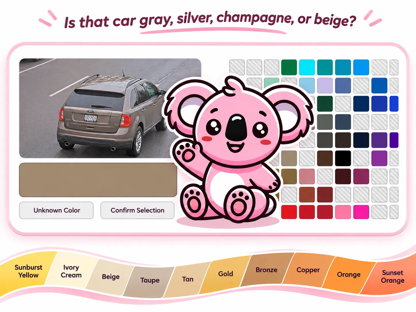
First, vehicle colors.
Is that car gray, silver, champagne, or beige?
We needed meaningful color names linked to RGB reference values, with a consistent way to map detailed colors into simpler categories.
Existing palettes, including CSS colors and industry-specific conventions, offered useful starting points. But no single universally accepted standard solved our problem.
We ended up developing the Pink Koala color palette: 55 named colors, also used in the labeling UI. The system also supports the NCIC color palette, used by the FBI and many insurance companies, as well as proprietary customer palettes.
Then, vehicle makes and models.
This was arguably even trickier.
The same car can have different names in different countries. Different models can look almost identical, while successive generations of one model can look completely different.
Should visually identical vehicles with different market names be separate classes? How should generations be handled? What distinctions can a model realistically learn from traffic-camera images?
These decisions have consequences. Splitting visually indistinguishable vehicles into separate classes can create contradictory training labels. Merging too many classes, on the other hand, sacrifices useful distinctions.
After reconciling data sources, naming conventions, and visually similar models, we arrived at a taxonomy of 521 make/model categories, including 467 specific categories and 54 “Other Models” categories.
Why did both AIs underestimate this work so substantially? One possibility is that their estimates implicitly treated classification labels as largely predefined. In our project, deciding what those labels should mean was a significant part of the engineering.
Before teaching AI to recognize something, you first need to define what that something is.
And that definition affects everything downstream: data collection, human annotation, model training, evaluation, and ultimately the predictions customers receive.
The takeaway
The lesson isn’t that AI estimates are unreliable, or that every computer vision project will follow the same distribution.
It’s that the difficulty of an AI project often lies somewhere other than where you expect it.
Here, model architecture accounted for just 4% of the effort, while taxonomy design consumed 15%. In another project, the proportions could be completely different.
One practical lesson we’d take into the next project: investigate taxonomy and labeling requirements early, rather than assuming the categories are already settled.
Building useful AI isn’t just about knowing how to train a model. It’s about knowing what the model should learn in the first place.
If you’re planning a computer vision project, we’d be happy to help identify its hidden challenges before they become expensive surprises.
Methodology: How we compared the estimates
We used Total Variation Distance (TVD), a standard measure for comparing two distributions.
For each of the ten individual categories, we calculated the absolute difference between actual effort and predicted effort, added those differences, and divided by two:
Here, Ai is the actual percentage and Pi is the predicted percentage for category i.
The factor of one-half prevents double-counting: effort overallocated to one category must be underallocated elsewhere.
Allocation overlap = 100% − TVD
We also included an equal-allocation baseline of 10% per category.
The table’s final column uses a simpler category-level measure:
Where Ci and Li are ChatGPT’s and Claude’s estimates. Section gaps are calculated from their subtotals.
This comparison is based on one project, retrospectively categorized tracked time, and two context-informed AI estimates. It isn’t a controlled study of model forecasting capabilities. The percentages describe allocations of effort, not absolute project duration or cost.